[1]:
%load_ext lab_black
Two parameter inference
This example illustrates parameter inference for the discount factor \(\delta\) and the wage constant in sector a for the setting of Keane-Wolpin (1994).
In this example the following moduels from respyabc are used:
Distance function for the descriptives:
distances.compute_mean_squared_distanceGet point estimate from inference:
evaluation.compute_point_estimatePlot credibility intervals from inference:
evaluation.plot_credible_intervalsPlot posterior distribution from inference:
evaluation.plot_kernel_density_posteriorSimulation function of the model:
models.compute_modelInference function:
respyabc.respyabc
We can import the necessary classes and packages by
[2]:
import respy as rp
import numpy as np

import time

from respyabc.distances import compute_mean_squared_distance
from respyabc.evaluation import compute_point_estimate
from respyabc.evaluation import plot_credible_intervals
from respyabc.evaluation import plot_kernel_density_posterior
from respyabc.models import compute_model
from respyabc.respyabc import respyabc
from respyabc.tools import convert_time
Load the default settings
First, we load the settings from the first model in Keane-Wolpin (1994) using respy.
[3]:
params, options, data_stored = rp.get_example_model("kw_94_one")
The model consits of 4 choices sector a, sector b, schooling and staying at home. This yields 30 parameters within the model. In this tutorial, we only vary over the discount factor, which is in the standard parameterization \(\delta = 0.95\).
[4]:
delta_default = params.loc[("delta", "delta")]["value"]
constant_a_default = params.loc[("wage_a", "constant")]["value"]

f"The default value of delta is {delta_default}."
[4]:
'The default value of delta is 0.95.'
[5]:
f"The default value of the wage constant in sector a is {constant_a_default}."
[5]:
'The default value of the wage constant in sector a is 9.21.'
Simulate the true population
For clarification, we reassign the default values to show how values with other options can be simulated. For a more detaield description see the tutorial on one parameter. We can address the wage constant using a melted index from its multiindex in params.
[6]:
model_to_simulate = rp.get_simulate_func(params, options)
parameter_true = {"delta_delta": 0.95, "wage_a_constant": 9.21}
As for one parameter, the model is subsequently passed to respyabc’s compute_model function.
[7]:
np.random.seed(123)
pseudo_observed_data = compute_model(
    parameter_true,
    model_to_simulate=model_to_simulate,
    parameter_for_simulation=params,
    options_for_simulation=options,
    descriptives="choice_frequencies",
)
Set the pyABC parameters
We set the size of the pyABC samples to 500 and the maximum number of drawn populations to 10. The excact magnitudes in applications depend on the respective application.
[12]:
population_size = 500
max_nr_populations = 10
For the two parameter inference, we need to define one prior distribution for each parameter.
[13]:
minimum_epsilon = 0.05
delta_prior_low = 0.9
delta_prior_length = 0.09
wage_a_constant_prior_low = 9
wage_a_constant_prior_length = 0.6
parameters_prior = {
    "delta_delta": [[delta_prior_low, delta_prior_length], "uniform"],
    "wage_a_constant": [
        [wage_a_constant_prior_low, wage_a_constant_prior_length],
        "uniform",
    ],
}
respyabc inference
As distance, we used the mean squared distances of the choice frequencies of any period. After specifying all relevant parameters, inference is conducted by using the respyabc function. We keep track of the simulation time to give the user a first glimpse about the timing.
[14]:
np.random.seed(1234)
start_time = time.perf_counter()
history = respyabc(
    model=compute_model,
    parameters_prior=parameters_prior,
    data=pseudo_observed_data,
    distance_abc=compute_mean_squared_distance,
    descriptives="choice_frequencies",
    population_size_abc=population_size,
    max_nr_populations_abc=max_nr_populations,
    minimum_epsilon_abc=minimum_epsilon,
)
end_time = time.perf_counter()
/home/manuel/anaconda3/lib/python3.7/site-packages/respy/pre_processing/model_processing.py:104: UserWarning: All seeds should be different.
  warnings.warn("All seeds should be different.", category=UserWarning)
/home/manuel/anaconda3/lib/python3.7/site-packages/respy/pre_processing/model_processing.py:104: UserWarning: All seeds should be different.
  warnings.warn("All seeds should be different.", category=UserWarning)
/home/manuel/anaconda3/lib/python3.7/site-packages/respy/pre_processing/model_processing.py:104: UserWarning: All seeds should be different.
  warnings.warn("All seeds should be different.", category=UserWarning)
/home/manuel/anaconda3/lib/python3.7/site-packages/respy/pre_processing/model_processing.py:104: UserWarning: All seeds should be different.
  warnings.warn("All seeds should be different.", category=UserWarning)
/home/manuel/anaconda3/lib/python3.7/site-packages/respy/pre_processing/model_processing.py:104: UserWarning: All seeds should be different.
  warnings.warn("All seeds should be different.", category=UserWarning)
/home/manuel/anaconda3/lib/python3.7/site-packages/respy/pre_processing/model_processing.py:104: UserWarning: All seeds should be different.
  warnings.warn("All seeds should be different.", category=UserWarning)
/home/manuel/anaconda3/lib/python3.7/site-packages/respy/pre_processing/model_processing.py:104: UserWarning: All seeds should be different.
  warnings.warn("All seeds should be different.", category=UserWarning)
[15]:
delta_time, delta_unit = convert_time(end_time - start_time)
f"The respyabc run for delta using choice frequencies took {delta_time:0.2f} {delta_unit}"
[15]:
'The respyabc run for delta using choice frequencies took 17.92 minutes'
respyabc evaluation
First, we compute the point estimate and its variance for both parameters. The estimate is computed by point_estimate as a weighted average over the latest simulated population.
[16]:
estimate = compute_point_estimate(history)
estimate
[16]:
| name | delta_delta | wage_a_constant |
|---|---|---|
| estimate | 9.348694e-01 | 9.126213 |
| est_variance | 3.141319e-07 | 0.000009 |
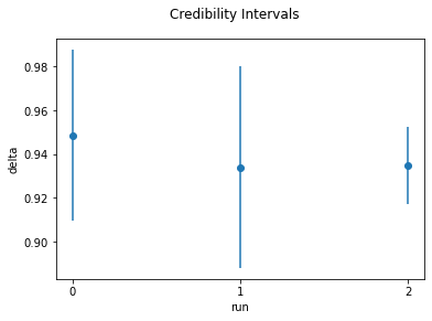
To obtain a broader overview on how the estimates evolve over the runs, we have implemented \(95\%\) credibility intervals by the function plot_credible_intervals. The argument interval_type=simulated indicates that the credibility intervals are computed as \(2.5\%\) and \(97.5\%\) percentiles of the simulated population. We do so for both parameters.
[17]:
plot_credible_intervals(
    history=history,
    parameter="delta_delta",
    interval_type="simulated",
    alpha=0.05,
    main_title="Credibility Intervals",
    y_label="delta",
)
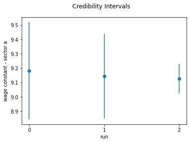
[18]:
plot_credible_intervals(
    history=history,
    parameter="wage_a_constant",
    interval_type="simulated",
    alpha=0.05,
    main_title="Credibility Intervals",
    y_label="wage constant - sector a",
)
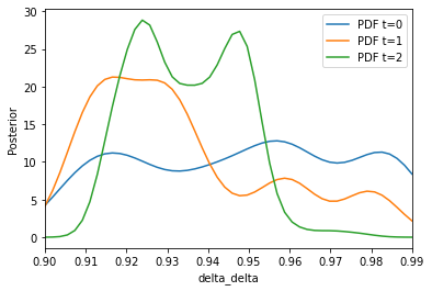
Computing the posterior distributions can be done analogously by plot_kernel_density_posterior and specifying the respective argument for parameter.
[19]:
xmax_delta = delta_prior_low + delta_prior_length
plot_kernel_density_posterior(
    history=history, parameter="delta_delta", xmin=delta_prior_low, xmax=xmax_delta
)
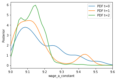
[20]:
xmax_constant = wage_a_constant_prior_low + wage_a_constant_prior_length
plot_kernel_density_posterior(
    history=history,
    parameter="wage_a_constant",
    xmin=wage_a_constant_prior_low,
    xmax=xmax_constant,
)
[ ]: